Searching for Incumbent Stability
I often use the birdnest simulator to test incumbents' stability against mutant invasion for certain games of interaction. For example, we might ask ourself, given that reproduction success is influenced by a public goods pairwise interaction, which public goods contribution is stable, given the following graph of contributions.
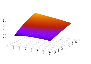
There are pretty straightforward methods to analytically compute stable incumbents, but it's much tricker to do this in an agent-based simulation. Let's start with the obvious problem: if we're computing stability of an incumbent against mutants, we need to check against enough mutants to make the numbers reasonable. Take, for example, the above matrix, and scan over the region [2, 3] in steps of 0.1.
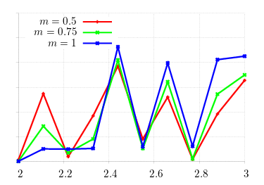
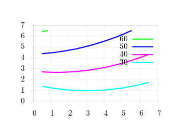
We know that stable incumbents lie in this region for the given values of m (the probability that offspring emigrate): as m increases, stability (small y-values) should slide from right to left. Obviously, the graph is way off the mark! We know the machinery is correctly working: what happens when we expand the search space?
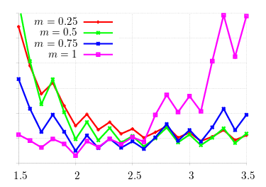

Better, but not good enough. I first ran a larger count of mutation runs (in theory, increasing precision), but the difference was negligable. What remains is to expand the search space. Unfortunately, the search space expands exponentially; and as it was, generating these values of m took on the order of 12 hours. Consider that the domain of 6 (i.e., [0.5, 6.5]) is divided into 10 unit steps. Given each incumbent checked against all other mutants, this amounts to 3600 checks. I then turned to the machinery generating the values, lsearch(1), which calls sp(1) for each incumbent/mutant configuration.
The lsearch(1) accepts a square payoff matrix (public goods contribution effects, for this example), splices it into incumbent and mutant, and runs each configuration in sequence. Like most other birdnest utilities, lsearch(1) uses MPI to parallelise mutations runs over processors. Specifically, mutation runs for each configuration are striped over processors (one to the first processor, two to the second, then onwards, wrapping from the maximum processors to the first). This works well with many mutation runs or generations, but for our needs, might be overkill.
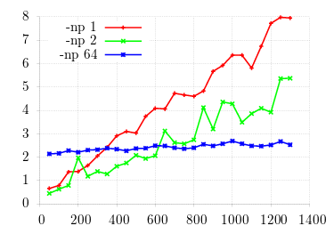
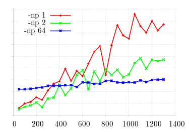
This simulation shows three different values of processor count for OpenMPI on a 64-core
machine.
Obviously we can, for a certain number of mutation runs and time horizon, outperform the full machine
version with a
single processor!
What if we can take advantage of the full machine with each processor running its own configuration?
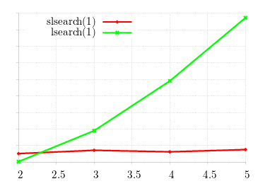
The results are excellent: while lsearch(1) run-time grows linearly
with matrix size, the new tool stays constant.
This tool, slsearch(1), round-robin distributes configurations to
processors.
It uses the poll() function to drain output from running processes, reaps then when finished, then
starts new processes in lieu of the old.
This maximises single-runs over the whole machine.
Obviously, when the matrix size exceeds the number of processors, the configuration time will increase; however, the graph will
rise step-wise with the number of available processors; not linearly with the matrix size.